Week 3
In this lesson, we learn about the data structures, encodings, and schemas used to store data and data indexes.
Objectives
After completing this week, you should be able to:
- Compare indexing algorithms including hash indexes and B-Trees
- Determine use cases for different methods of organizing data including column-oriented storage and snowflake schemas
- Make use of different encoding formats including Avro, Thrift, JSON, XML, and Protocol Buffers
- Describe the different methods of using data schemas including schema-on-read, schema-on-write, and different methods of schema evolution
Readings
- Read chapters 3 and 4 in Designing Data-Intensive Applications
Weekly Resources
Assignment 3
For this assignment, you will be working with data from OpenFlights. This data was originally obtained from the OpenFlights Github repository and a copy of the original data is found in data/external/openflights/. For this assignment, you will use a dataset derived from that original data. You can find this data in data/processed/openflights/routes.jsonl.gz. The data is compressed with gzip and encoded in the JSON Lines format. Each line represents a single airline route.
The dsc650/assignments/assignment03 directory contains placeholder code and data outputs for this assignment.
Assignment 3.1
In the first part of the assignment, you will be creating schemas for the route data and encoding the routes.jsonl.gz using Protocol Buffers, Avro, and Parquet.
a. JSON Schema
Create a JSON Schema in the schemas/routes-schema.json file to describe a route and validate the data in routes.jsonl.gz using the jsonschema library.
b. Avro
Create an Avro schema in the schemas/routes.avsc file to describe a route and validate the data in routes.jsonl.gz. Use Avro's Python library or fastavro library to create results/routes.avro with the schema you created. Do not use any compression on the output at this stage.
c. Parquet
Create a Parquet dataset in results/routes.parquet using Apache Arrow and Pandas. Do not use any compression on the output at this stage.
d. Protocol Buffers
Define a Protocol Buffers message format in schemas/routes.proto. Using the Protocol Buffers Python tutorial as a guide, compile the routes.proto into Python classes. Output the generated code into dsc650/assignment/assignment03/routes_pb2.py. Use this generated code to create results/routes.pb using Protocol Buffers. Do not use any compression on the output at this stage.
e. Output Sizes
Compare the output sizes of the different formats. Populate the results in results/comparison.csv.
Assignment 3.2
This part of the assignment involves developing a rudimentary database index for our routes dataset. Filesystems, databases, and NoSQL datastores use various indexing mechanisms to speed queries.
The implementation of advanced data structures such as B-Trees, R-Trees, GiST, SSTables, and LSM trees is beyond the scope of this course. Instead, you will implement a rudimentary geospatial index using geohashes and pygeohash.
Without going into too much detail, a geohash converts geospatial coordinates (i.e. latitude and longitude) into single, usually, base64 or base32 encoded integer. Below is an example of the geohashed value for Bellevue University.
import pygeohash
pygeohash.encode(41.1499988, -95.91779)
'9z7f174u17zb'
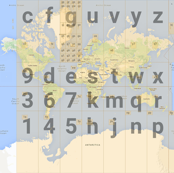
Geohashes have the useful property that when they are sorted, entries that are near one another in the sorted list are usually close to one another in space. The following image shows how this gird looks.

The following table gives cell width and height values for each level of precision of the geohash.
| Geohash | Coordinates | Cell Width1 | Cell Height |
|---|---|---|---|
| 9 | 22.0, -112.0 | ≤ 5,000km | 5,000km |
| 9z | 42.0, -96.0 | ≤ 1,250km | 625km |
| 9z7 | 41.0, -96.0 | ≤ 156km | 156km |
| 9z7f | 41.0, -96.0 | ≤ 39.1km | 19.5km |
| 9z7f1 | 41.2, -95.9 | ≤ 4.89km | 4.89km |
| 9z7f174u | 41.15, -95.918 | ≤ 38.2m | 19.1m |
| 9z7f174u17zb | 41.149999, -95.91779 | ≤ 4.77m | 4.77m |
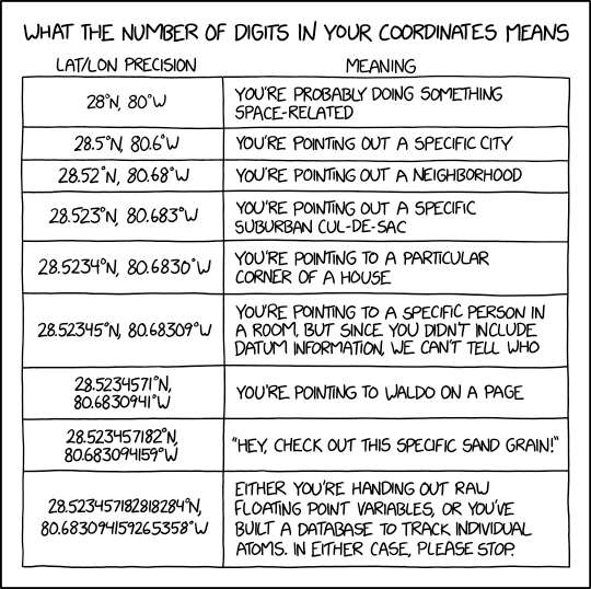
As you can see, it only takes about four levels characters to get to a 40 km by 20 km area. Another level gives 5 km by 5 km. In most cases, going past 12 units of precision is pointless as very few applications require that degree of accuracy.

a. Create a Simple Geohash Index
Using pygeohash create a simple index for the routes.jsonl.gz data using the source airport latitude and longitude. Output the index and values to the results/geoindex directory. The output looks like the following directory structure.
geoindex
├── 2
│   ├── 2e
│   │   ├── 2eg.jsonl.gz
│   │   ├── 2ev.jsonl.gz
│   │   └── 2ey.jsonl.gz
│   ├── 2h
│   │   ├── 2h5.jsonl.gz
│   │   ├── 2hb.jsonl.gz
│   │   └── 2hx.jsonl.gz
│   ├── 2j
│   │   ├── 2j0.jsonl.gz
│   │   ├── 2j3.jsonl.gz
│   │   ├── 2jd.jsonl.gz
.
.
.
│   └── yu
│       └── yue.jsonl.gz
└── z
    ├── z0
    │   ├── z08.jsonl.gz
    │   ├── z0h.jsonl.gz
    │   └── z0m.jsonl.gz
    ├── z6
    │   └── z6e.jsonl.gz
    ├── z9
    │   └── z92.jsonl.gz
    ├── zg
    │   └── zgw.jsonl.gz
    ├── zk
    │   └── zk9.jsonl.gz
    ├── zs
    │   └── zs4.jsonl.gz
    └── zu
        └── zu3.jsonl.gz
b. Implement a Simple Search Feature
Implement a simple geospatial search feature that finds airports within a specified distance of an input latitude and longitude. You can use the geohash_approximate_distance function in pygeohash to compute distances between geohash values. It returns distances in meters, but your search function should use kilometers as input.
import pygeohash
pygeohash.geohash_approximate_distance('bcd3u', 'bc83n')
# >>> 625441
c. Evolve the Protocol Buffers and Avro Schemas
Protocol Buffers, Avro, and Parquet all allow for schema evolution. Create an updated Avro schemas that include the field geohash for source and destination airports. Create this in the schemas directory as routesv2.avsc. Use this new schema to validate the previously created routes.avro dataset. If you evolved your schema correctly, the new schema should be backward compatible.
Submission Instructions
For this assignment, you will submit a zip archive containing the contents of the dsc650/assignments/assignment03/ directory. Use the naming convention of assignment03_LastnameFirstname.zip for the zip archive. You can create this archive in Bash (or a similar Unix shell) using the following commands.
cd dsc650/assignments
zip -r assignment03_DoeJane.zip assignment03
Likewise, you can create a zip archive using Windows PowerShell with the following command.
Compress-Archive -Path assignment03 -DestinationPath 'assignment03_DoeJane.zip
When decompressed, the output should have the following directory structure.
├── __init__.py
├── results
│   ├── comparison.csv
│   ├── geoindex
│   ├── routes.avro
│   ├── routes.parquet
│   ├── routes.pb
│   └── validation-results.csv
├── routes_pb2.py
├── routesv2_pb2.py
├── run_assignment.py
├── schemas
│   ├── routes-schema.json
│   ├── routes.avsc
│   ├── routes.proto
│   ├── routesv2.avsc
│   └── routesv2.proto
└── util.py
Your assignment may also contain additional files depending on you choose to implement your code.
Discussion
For this discussion, pick one of the following topics and write a 250 to 750-word discussion board post. Use the DSC 650 Slack channel for discussion and replies. For grading purposes, copy and paste your initial post and at least two replies to the Blackboard discussion board.
Topic 1
Describe a real-world use case for snowflake schemas and data cubes. In particular, why would you want to use a snowflake schema instead of the presumably normalized schemas of an operational transactional database?
Topic 2
Parquet is a column-oriented data storage format, while Avro is a row-oriented format. Describe a use case where you would choose a column-oriented format over a row-oriented format. Similarly, describe a use case where you would choose a row-oriented format.
Topic 3
Describe the trade-offs associated with different data compression algorithms. Why would one choose a compression algorithm like Snappy over an algorithm like Gzip or Bzip2? Should you use these algorithms with audio or video data? How should you use compression with encrypted data?
Topic 4
We briefly talked about different data indexing strategies including B-Trees, LSM trees, and SSTables. Provide examples of other data indexing algorithms and how you might use them in a production environment.
-
Cell width and height numbers taken from https://www.movable-type.co.uk/scripts/geohash.html ↩